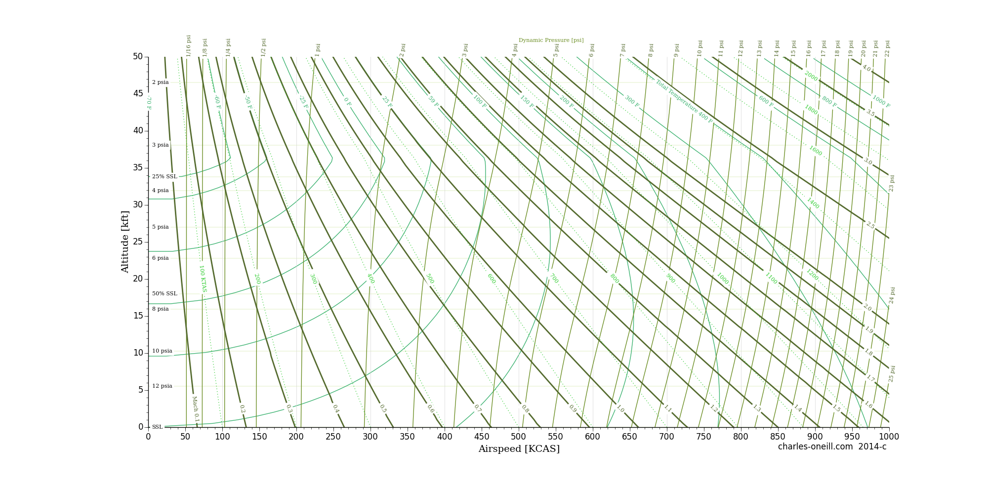
This post provides a visual characterization of a generic flight envelope with a standard atmosphere. The following figure shows a generic flight envelope map.
Atmosphere and Airspeed
A pdf version is available at airspeed-2014c.pdf. This file plots altitude (0 to 50 thousand feet), calibrated airspeed (0 to 1000 KCAS), true airspeed, Mach number, dynamic pressure, static pressure, and total temperature on one handy page.
Airspeed:
Engineers and pilots track three different speeds:
- Calibrated Airspeed: the airspeed from the pitot system corrected for instrument bias
- True Airspeed: actual speed through the air
- Groundspeed: speed referenced to level ground
We will only be concerned with calibrated airspeed (KCAS: knots calibrated airspeed) and true airspeed (KTAS: knots true airspeed). For reference, a knot [kt] is 1.688 feet per second [ft/s].
The atmosphere is referenced to a standard atmospheric model (see U.S. Standard Atmosphere). The ratios of properties are convenient:
$$\delta=\frac{p}{p_{ssl}}$$
$$ \theta=\frac{T}{T_{ssl}}$$
$$\sigma=\frac{\rho}{\rho_{ssl}} = \frac{\delta}{\theta}$$
From compressible flow theory, an isentropic process gives a stagnation pressure (aka. total pressure) of $$p_{t}=p\left(1+\frac{\gamma-1}{2}M^{2}\right)^{\frac{\gamma}{\gamma-1}}$$
Rearranging with $$V=aM$$
and $$\Delta p=p_{t}-p$$
results in $$V^{2}=\frac{2a^{2}}{\gamma-1}\left[\left(\frac{p_{t}}{p}\right)^{\frac{\gamma-1}{\gamma}}-1\right]$$
which is identical to $$V^{2}=\frac{2a^{2}}{\gamma-1}\left[\left(\frac{\Delta p}{p}+1\right)^{\frac{\gamma-1}{\gamma}}-1\right]$$
Rearranging gives $$\frac{p_{t}}{p}\frac{p}{p_{ssl}}=\left(\frac{V^{2}}{a_{ssl}^{2}}\frac{\gamma-1}{2}+1\right)^{\frac{\gamma}{\gamma-1}}$$
Substitution gives $$\frac{p_{t}}{p}=\frac{1}{\delta}\left(\frac{V^{2}}{a_{ssl}^{2}}\frac{\gamma-1}{2}+1\right)^{\frac{\gamma}{\gamma-1}}$$
Mach Meter
A Mach meter determines the freestream mach number from a pressure ratio. $$M=\sqrt{\frac{2}{\gamma-1}\left[\left(\frac{p_{t}}{p}\right)^{\frac{\gamma-1}{\gamma}}-1\right]}$$
or the inverse $$\frac{p_{t}}{p}=\left(M^{2}\frac{\gamma-1}{2}+1\right)^{\frac{\gamma}{\gamma-1}}$$
However, when the upstream Mach number exceeds 1, a shock will be generated forward of the pitot tube. Given the freestream is point 1 and the pitot is point 3, the pressure ratio upstream in terms of the shock’s M
are $$\frac{p_{t_{1}}}{p_{1}}=\left(\frac{p_{t_{3}}}{p_{1}}\right)\left(\frac{p_{t_{1}}}{p_{t_{3}}}\right)$$
Where from compressible flow of a shock, the stagnation pressure ratios are $$\left(\frac{p_{t_{3}}}{p_{t_{1}}}\right)=\left(\frac{\frac{\gamma+1}{2}M_{1}^{2}}{1+\frac{\gamma-1}{2}M_{1}^{2}}\right)^{\frac{\gamma}{\gamma-1}}\left(\frac{2\gamma}{\gamma+1}M_{1}^{2}-\frac{\gamma-1}{\gamma+1}\right)^{\frac{-1}{\gamma-1}}$$
Substitute into $$\frac{p_{t_{1}}}{p_{1}}=\left(M^{2}\frac{\gamma-1}{2}+1\right)^{\frac{\gamma}{\gamma-1}}$$
giving $$\left(\frac{p_{t_{3}}}{p_{3}}\right)=\left(M^{2}\frac{\gamma-1}{2}+1\right)^{\frac{\gamma}{\gamma-1}}\left(\frac{p_{t_{3}}}{p_{t_{1}}}\right)$$
which is $$\left(\frac{p_{t_{3}}}{p_{3}}\right)=\left(M_{1}^{2}\frac{\gamma-1}{2}+1\right)^{\frac{\gamma}{\gamma-1}}\left(\frac{\frac{\gamma+1}{2}M_{1}^{2}}{1+\frac{\gamma-1}{2}M_{1}^{2}}\right)^{\frac{\gamma}{\gamma-1}}\left(\frac{2\gamma}{\gamma+1}M_{1}^{2}-\frac{\gamma-1}{\gamma+1}\right)^{\frac{-1}{\gamma-1}}$$
This reduces to the Reighleigh Pitot Equation $$\left(\frac{p_{t_{3}}}{p_{3}}\right)=\left(\frac{\gamma+1}{2}M_{1}^{2}\right)^{\frac{\gamma}{\gamma-1}}\left(\frac{2\gamma}{\gamma+1}M_{1}^{2}-\frac{\gamma-1}{\gamma+1}\right)^{\frac{-1}{\gamma-1}}$$
Given a particular pressure ratio, only one Mach number satisfies this equation. Even better, the subsonic value is a good approximation for this supersonic value.
Calibrated Airspeed
The airspeed indicator operates by receiving static pressure from a static port and stagnation pressure from a pitot system. The airspeed indicator measures the pressure difference: $$\Delta p=p_{t}-p_{static}$$
The reference pressure and speed of sound are the sea level values. $$V_{cal}=\sqrt{\frac{2a_{ssl}^{2}}{\gamma-1}\left[\left(\frac{\Delta p_{cal}}{p_{ssl}}+1\right)^{\frac{\gamma-1}{\gamma}}-1\right]}$$
The inverse mapping indicates the pressure differential generated for a given calibrated airspeed. $$\Delta p_{cal}=p_{ssl}\left[\left(\frac{\gamma-1}{2}\left(\frac{V_{cal}}{a_{ssl}}\right)^{2}+1\right)^{\frac{\gamma}{\gamma-1}}-1\right]$$
Subsonic Case (ONLY):
For the subsonic case only, computing the true airspeed simplifies to an explicit equation. From the calibrated airspeed, we found a pressure differential. This pressure differential is applied to the same stagnation pressure relation for the local properties. $$V_{true}=\sqrt{\frac{2a^{2}}{\gamma-1}\left[\left(\frac{\Delta p_{cal}}{p}+1\right)^{\frac{\gamma-1}{\gamma}}-1\right]}$$
Thus the ratio of true to calibrated airspeed is $$\frac{V_{true}}{V_{cal}}=\sqrt{\frac{\frac{2a^{2}}{\gamma-1}\left[\left(\frac{\Delta p_{cal}}{p}+1\right)^{\frac{\gamma-1}{\gamma}}-1\right]}{\frac{2a_{sl}^{2}}{\gamma-1}\left[\left(\frac{\Delta p_{cal}}{p_{ssl}}+1\right)^{\frac{\gamma-1}{\gamma}}-1\right]}}$$
Cancelling terms gives with $$a^{2}=\gamma RT$$
gives $$\frac{V_{true}}{V_{cal}}=\sqrt{\theta\frac{\left[\left(\frac{\Delta p_{cal}}{p_{ssl}}\frac{1}{\delta}+1\right)^{\frac{\gamma-1}{\gamma}}-1\right]}{\left[\left(\frac{\Delta p_{cal}}{p_{ssl}}+1\right)^{\frac{\gamma-1}{\gamma}}-1\right]}}$$