Landing on Mars is a difficult engineering problem. A recent conceptual project demonstrated this reality through the atmospheric reentry profile. In other words, assuming that your spacecraft approaches Mars at 200 kilometers and 6.5 kilometers per seconds, what is the altitude-velocity profile during the reentry trip?

Complicating the situation is an observation that your vehicle’s aerodynamics strongly affect the profile. In particular, increasing the life decreases the observed g-load, but leads to atmospheric skip when the lift is not controlled.

A ballistic reentry vehicle should expect a maximum g-load above 10 in the 50 km altitude region. This conceptual analysis strongly suggests that manned reentry to Mars will require hypersonic aerodynamics generation of a lift over drag (L/D) ratio in the 0.5 range.

The graduate level AEM 614 Wing and Airfoil Theory class at the University of Alabama was resurrected, developed, and taught in the fall of 2015.

The course used two textbooks:

Flight Vehicle Aerodynamics, Mark Drela, MIT Press, 2014
Aerodynamic Design of Transport Aircraft, Ed Obert, IOS Press, 2009

Student Evaluations: 15Charles O’Neill (AEM 614-001 Airfoil And Wing Theory)

Aerospace engineers encounter vortex methods as undergraduates. The famous thin airfoil theory is a continuous vortex sheet. The famous XFOIL is a panel method with an IBL solver for viscous effects.

Q: Can a simple discrete vortex method capture thickness?

A: Yes, but I would recommend a linear vortex method instead.

The source code and executable are available here.

The visualization is a pure Fortran library exporting to scalable vector graphics (.svg).

 

\(\)In the spring, a colleague asked a question regarding the computation of circulation about an airfoil. In response, I created a comparison of methods to calculate the circulation about an NACA 0012 airfoil at 10 degrees angle of attack, Mach 0.16 and a Reynolds number of 6 million. Data was generated with the FUN3D CFD solver with an SA turbulence model. The visualization is through TecPlot360. The pressure coefficient, \(C_p \), field is given below:

The definition of vorticity is: $$ \omega = \nabla\times V$$ In 2D, expanding gives $$\omega = \frac{dV_y}{dx} – \frac{dV_x}{dy} $$Computing the vorticity in the domain gives the following field.

Three methods will be used to determine the circulation \(\Gamma \) about the airfoil.

• Method 1: Compute from lift coefficient. The CFD solver estimates a lift coefficient of 1.09. From the Kutta-Joukowski theorem, lift per unit span is proportional to circulation. Solving for circulation gives $$ \Gamma = \frac{1}{2} V_o \rho C_l $$ Computing gives \(\Gamma = 1.04 \)
• Method 2: Integrate vorticity in domain. $$\Gamma = \int\int_A \omega dA $$ Computing gives \(\Gamma = 1.03 \)
• Method 3: Contour integral of velocity. A coarse numerical integral with 16 points manually sampled from the CFD computed velocity components \[\Gamma  =  – \oint\limits_S {V \cdot ds} \]. This computation gives a circulation of \(\Gamma = 1.01\).

 

---

Calculator:

Inputs
Pressure [psi]
Temperature [F]
Relative Humidity [%]
Calculated
Density [slug/ft3]
Density Alt [ft]

---

Theory:

Warning: Don’t make this fundamental error in determining the density of moist air.

Recently, I’ve been preparing a graduate level course on Wing and Airfoil Theory. One lecture delves into modeling the real atmosphere including humid, wet, moist air. Specifically, I wanted to calculate the density of humid air. Visit my Atmosphere page for more information and tools.

[Update 1st March 2019] A moist air density calculator is at the top of this page.

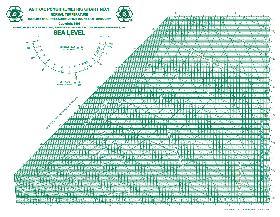
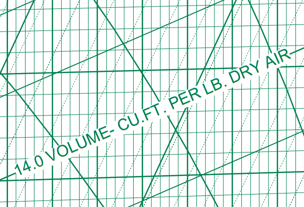
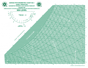
My first thought was to grab a psychometric chart from my wife’s ASHRAE handbook which is available in pdf format at: ASHRAE Psychometric Chart No. 1The chart plots lines of density, dry-bulb temperature, wet-bulb temperature, enthalpy, and relative humidity. As an example, at 90 F and 90% relative humidity, the chart indicates a volume per cubic foot of dry air of approximately 14.48. This gives a density of 0.00214 slugs per cubic foot.

However, this density is not the density of humid air. I didn’t catch the mistake until verifying my own independent calculating routine.

\(\) My derivation started with an ideal gas approximation of dry air and water vapor. The total pressure \(p\) is the summation of partial pressures for dry air \(p_d\) and water vapor \(p_w\).

$$\rho = \frac{p_d}{R_d T_d}+\frac{p_v}{R_v T_v}$$

Since the temperatures are identical, the density is:

$$\rho = \frac{p_d M_d + p_v M_v}{\bar R T}$$

Given that the relative humidity relates the partial pressure of water vapor to the saturation pressure of water pressure \(p_v = \phi p_s \), the density formula is rearranged to

$$\rho = \frac{p M_d + \phi p_s \left(  M_v – M_d \right)}{\bar R T}$$

Since the molecular mass weight of dry air is \( 28.97 \frac{lbm}{lbmol} \) while water vapor is lower at \( 18.00 \frac{lbm}{lbmol} \), the density of wet air is always lower than dry air.

The reduction in magnitude depends on the saturation pressure of water vapor. For the region of interest to aerodynamics, the Arden-Buck equation provides a curve fit approximation to the partial pressure of water vapor. Converted to standard units, the partial pressure in psi given a temperature in R is:

$$p_s(T) = 0.08865 \exp\left(\frac{-0.002369 (T-8375.65)(T-491.67)}{T-28.818}\right)$$

Combining the density and partial pressure formulas gives an alternative estimate of the density of air at 90 F and 90% humidity of 0.002203 slugs per cubic foot.

So what gives? Who is correct? Why is the gold-standard ASHRAE chart suggesting a lower density? The key words are: volume per cubic foot of dry air.

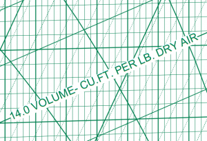
The ASHRAE chart gives the density of only the air and NOT the water vapor. The ASHRAE chart clearly states that only the dry air component is considered.

Adding in the water vapor requires finding the humidity ratio.

For the 90 F and 90% case, the humidity ratio is 0.028. Each 100 pounds of dry air has 2.8 pounds of water. Correcting the previous ASHRAE density gives:

$$ \rho = (1+0.028) 0.00214 \frac{slugs}{ft^3} $$ which is 0.002207 slugs per cubic foot.

Mystery solved.

Warning: There are websites out there inadvertently giving the wrong density of wet air. One example is denysschen.com. A single sentence would correct the confusion. On the other hand, the site at hvac-calculator.com appears to give the correct value.

I successfully retrieved my Liebelle glider from the top of a 30 foot tall tree. I recommend this method over pulling the plane down through the tree with string.

Here are the supplies:

1. Extendable painter’s pole (23 foot available at Homedepot)
2. A tall drinking cup to capture the glider’s forward fuselage
3. Duct tape to connect the mug to the pole
4. A helper to grab the plane off the pole

The requirements were specific. I didn’t want to destroy the plane. The tree was too small to climb; the plane was in the top branch. The solution was to lift the plane out vertically with the pole.

 

Lessons learned:

1. Some fields are even too small for 1.1 meter DLG flying
2. My distance/height estimation was not tuned to a 1.1 meter glider. I flew it directly into a tree… CFIT (controlled flight into terrain tree)
3. Maneuvering a 8 to 24 foot pole up through tree limbs is not easy. I was lucky to have a small and sparsely branched tree.
4. Lifting the plane once connected was trivial and easy.
5. My helper was useful to support the pole and plane on the descent. This become necessary once the pole was angled.
6. Non destructive tree retrieval is feasible

I never met my first boss. This happened 15 years ago; the shock, the sadness, and his sister’s voice on the phone are still here. Thanks for the opportunity Mr. Carlson; I’m sorry that we never met.

From the NTSB accident report:

---

NYC00LA141
On May 24, 2000, about 0930 Eastern Daylight Time, a homebuilt Criquet, N22CA, was destroyed while departing Aero Flight Center Airport, East Palestine, Ohio. The certificated private pilot/owner was fatally injured. Visual meteorological conditions prevailed, and no flight plan was filed for the local personal flight conducted under 14 CFR Part 91.

 

A witness at the airport stated that the pilot initially performed a full power run-up, then shut the engine down. The pilot told the witness that the engine was producing 50 to 100 rpm less than maximum power. The pilot adjusted the carburetor, restarted the engine, and performed another run-up. During the second run-up, he checked both magnetos, but did not perform a full power run-up. The airplane then departed on Runway 29, a 3,000 foot long, 100 foot wide turf runway.

The witness added that the airplane usually used about “half the runway” to takeoff. On the accident flight, the airplane used about “three quarters of the runway.” It then made a right turn to avoid trees, but struck a tree with the right wing. The airplane came to rest inverted in a bean field, and a post crash fire ensued. While examining the wreckage with a Federal Aviation Administration (FAA) inspector, the witness stated that the supercharger appeared to be disengaged.

Another witness, who was a retired mechanic, stated that he was familiar with the airplane. The airplane’s engine was a Lom Praha M332AK, manufactured in the Czech Republic. Several months before the accident, the pilot noticed the engine was not producing maximum power. The mechanic examined the engine, and found a leak in the exhaust valve of a cylinder. The cylinder was repaired at a machine shop and reinstalled; however, the engine still did not produce maximum power.

The pilot eventually sent the engine back to the manufacturer for repair. While the engine was being repaired, the manufacturer provided the pilot with a “loaner” engine. The mechanic stated that the airplane performed much better with the “loaner” engine, and the pilot never had any problems.

The pilot’s original engine was returned without any paperwork. According to the mechanic, he and the pilot did not know what repairs were made to the engine. The pilot and mechanic reinstalled the original engine.

On the day of the accident, the pilot performed one run-up near his hangar. He performed a second run-up at the end of the runway that lasted approximately 20 minutes. The mechanic stated that the airplane used about “two thirds of the runway” for takeoff. As it became airborne, the engine “sounded ok,” but the airplane did not seem to have enough airspeed or altitude. It struck trees at the end of the runway and a fire ensued.

When asked about the lack of power, the mechanic stated that there might have been something wrong internally with the engine. He said that he wasn’t sure, but that the engine was “lazy.” When asked about the supercharger, the mechanic stated that the pilot may not have engaged it. He added that the supercharger didn’t make a noticeable difference when it was engaged or disengaged.

A Federal Aviation Administration inspector examined the wreckage. He stated that due to the post crash fire, he was unable to verify flight control continuity or conduct an engine examination.

The airplane was issued a temporary, 3 month, special airworthiness certificate on May 27, 1999, by a FAA inspector. After the certificate expired, and the original engine was reinstalled, no FAA inspector had examined the airplane.

At 0950, at an airport approximately 10 miles away, the reported wind was from 250 degrees at 15 knots.

The pilot’s most recent FAA third class medical certificate was issued on August 17, 1996. At that time, he reported a total flight experience of 2,000 hours. According to the airplane logbook, it had approximately 8 hours of operation.

Toxicological testing, conducted at the FAA Toxicology Accident Research Laboratory, Oklahoma City, Oklahoma, was negative for drugs and alcohol.

Continue reading →

My first, second, and third thermal! Finding and soaring in thermals is a new experience for me.

I’ve read the books (“Joy of Soaring”) , devoured the “Soaring” journal (back as an undergrad), and even tried to simulate a sailplane with a Cessna (lousy idea). However, yesterday was the first time that I’ve actually done so with an airplane capable of soaring.

The plane is a Dreamflight Libelle DLG.