Counterfeit Futaba servos exist. My students and I managed to purchase a few for a recent aircraft project. These were purchased off of Amazon. We now call these “Faketaba” servos.
Question: How many ways can you tell that the following servo is a counterfeit Futaba S3003 servo?
Answer:
- The servo performance is significantly worse than a genuine servo. In fact, I (Charles O’Neill) initially discovered that these servos were not genuine after performing a systems check of installed servos. The return to zero had a hysteresis of about several millimeters at the servo horn, which gave a surface deflection static hysteresis “zero” of about +-10 degrees. This was completely unacceptable for our application. These were immediately removed and replaced.
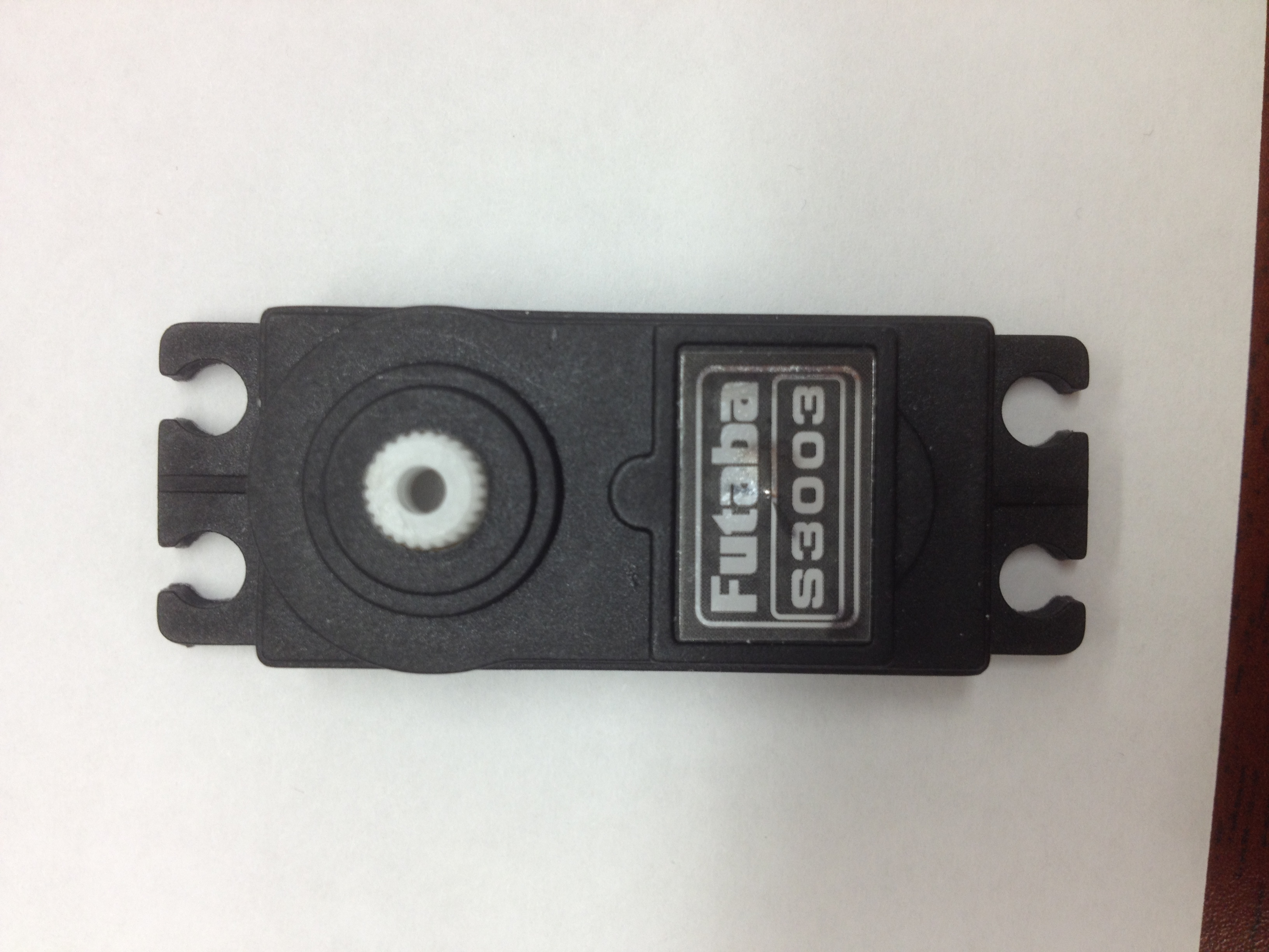
- The Futaba logo and font is not correct. As a typography enthusiast, I spotted the slight imperfections in the name sticker.
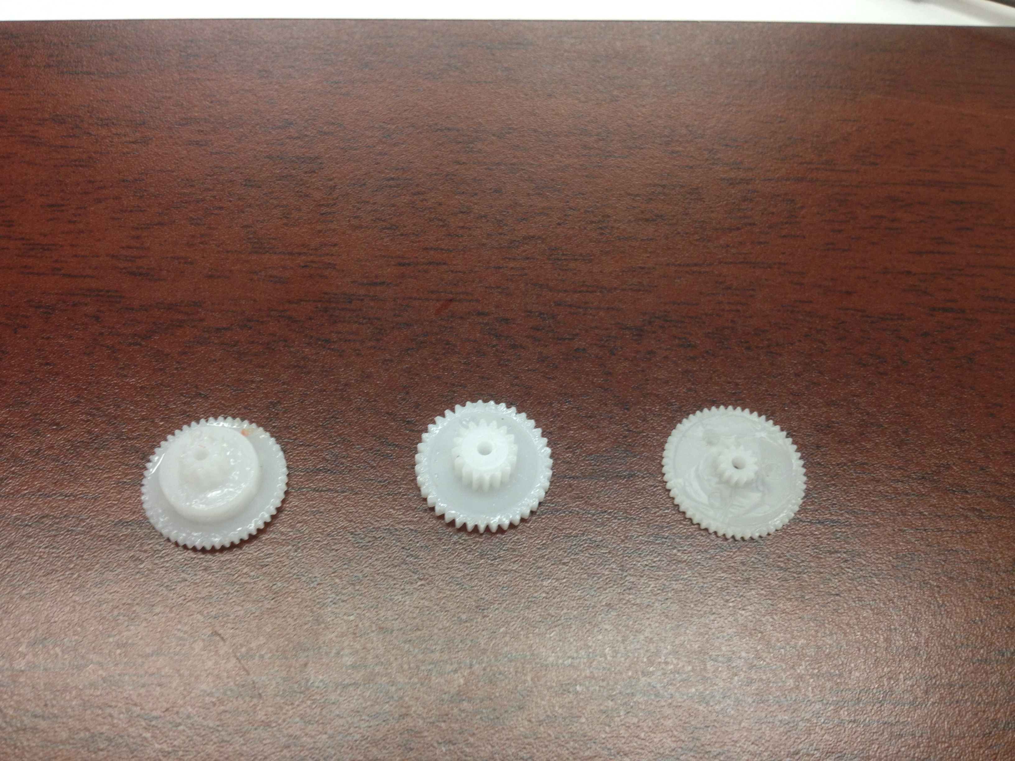
- Gear noise is sigificantly higher for these fake servos. The gear geometry and tooth count are different from actual Futaba servos.
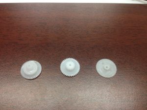
- In addition to the gear noise, the output shaft tolerance created an issue with the bearing surfaces. Also, the spline shaft poorly fit the servo horns. The servo horns themselves were significantly thicker than genuine horns.
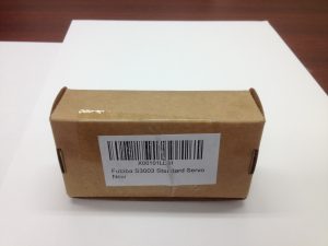
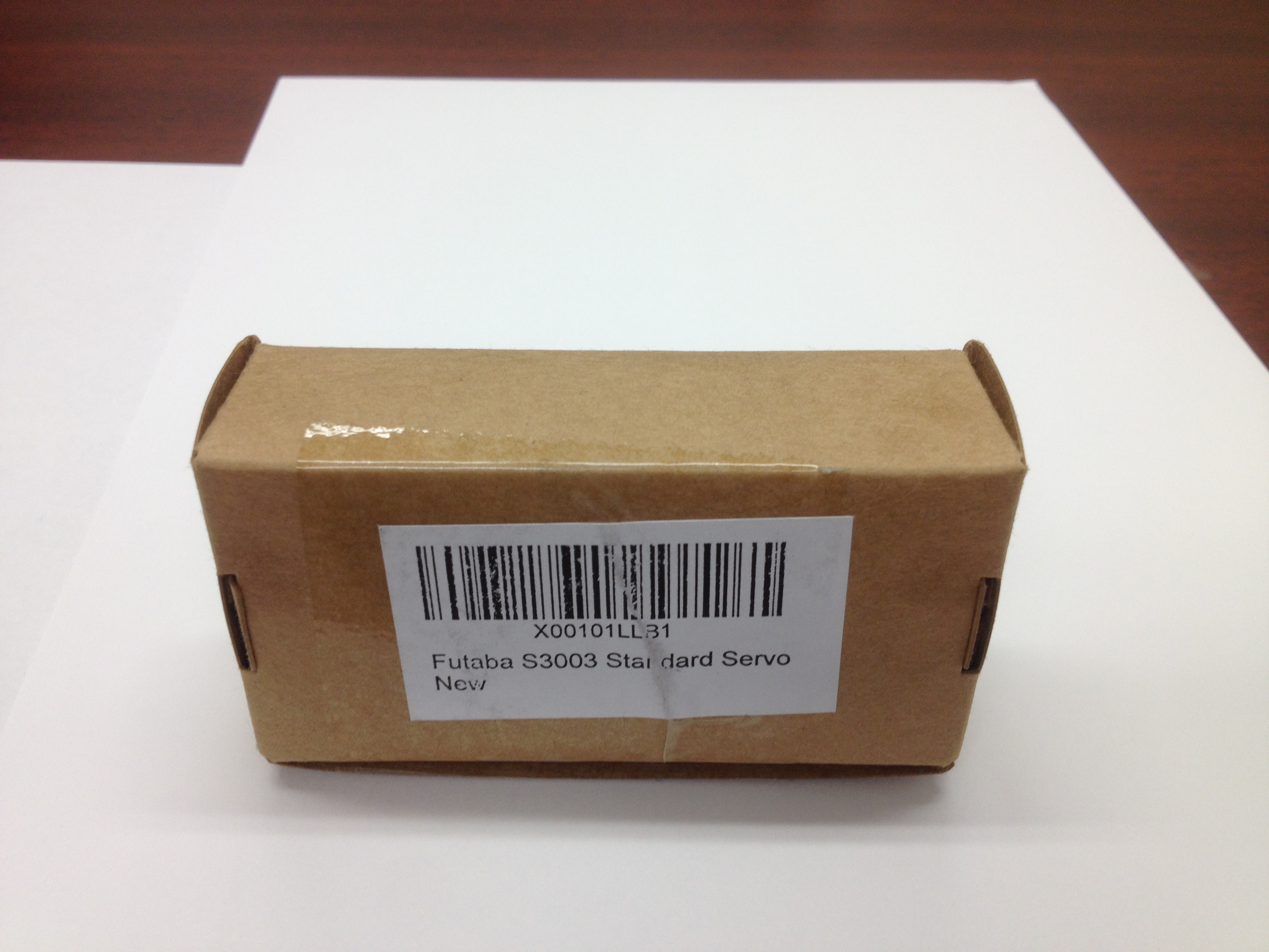
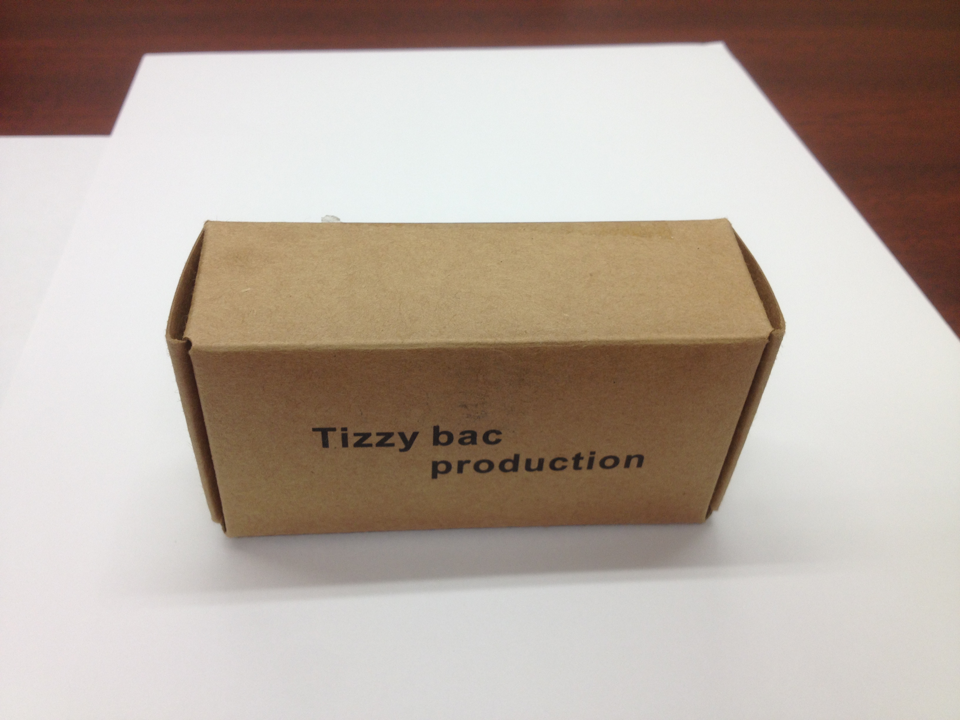
- After installation, I went back and found the box that the servos were shipped in. This is obviously not a genuine Futaba box.

- I opened one servo to investigate the counterfeit quality. The grommet was not sealed correctly, a mistake that the Japanese Futaba company would never allow. The motor is only press fit into the servo case; this is a sneaky possible failure point. The servo case is geometrically different from an actual case.
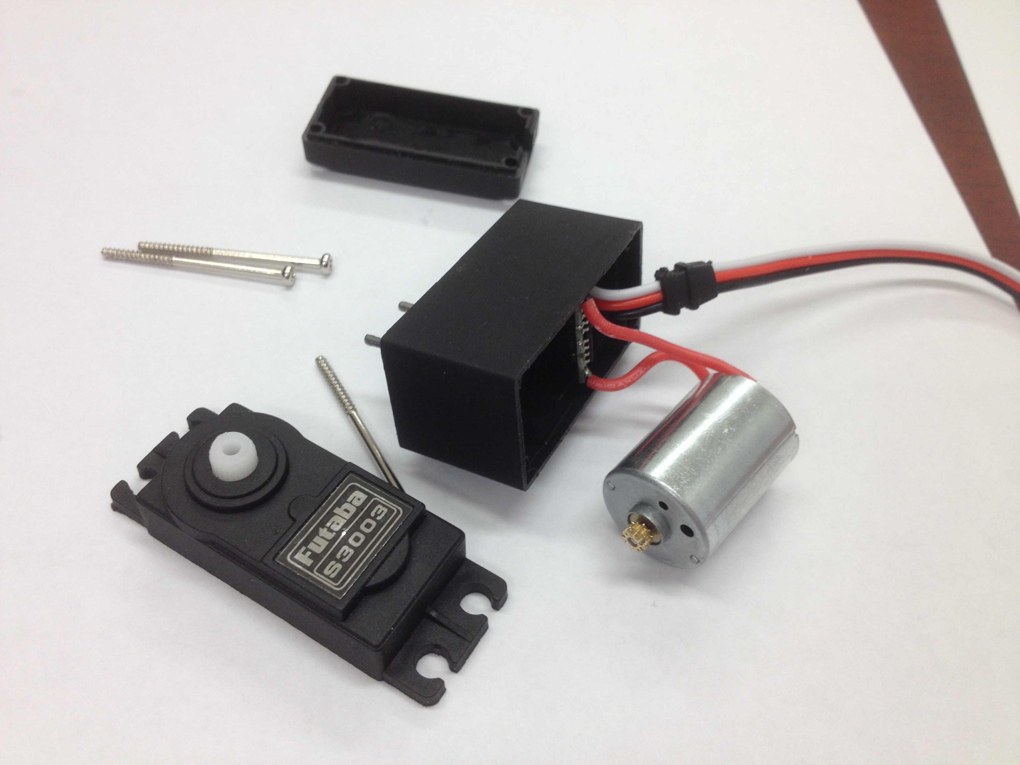
- The mounting holes are opened at the end. Actual Futaba S3003 servos are closed.
One additional point of discussion, the cost for these counterfeits was similar to actual genuine servos. My students learned a difficult lesson in trust.